Society of Exploration Geophysicists, 2014
Ground penetrating abilities of broadband pulsed radar in the 1 − 70MHz range
K. van den Doel∗, Univ. of British Columbia, J. Jansen, Teck Resources Limited, M. Robinson, G. C, Stove, G. D. C. Stove, Adrok Ltd
Summary
We describe underground experiments to quantify the penetration capabilities of broadband pulsed radar in the 1 − 70MHz range. A radar pulse was sent by trans illumination experiments through a limestone pillar ranging in thickness of limestone ranging from 17m to 121m and the losses were measured. The high frequencies were found to penetrate very little, but the low frequency component had very low losses. Results were analyzed to estimate the skin depth and interpreted in terms of a constitutive model incorporating Maxwell’s equations with conductivity and polarization losses.
In a second experiment we successfully detected the reflection of the radar pulse from a body of water through 350m of rock. A numerical simulation of the model confirmed that these results do not contradict theoretical expectations.
Introduction
Ground penetrating radar (GPR) is an active area of research with a plethora of applications, see for example (Jol, 2009) for a comprehensive overview. Its non-invasive nature and low cost make it a very attractive subsurface imaging technology. The major limitation for geophysical exploration applications is that ground penetration is constrained by electromagnetic losses, which are rather high in the commonly used frequency range of 10 − 1000MHz, resulting in a rather shallow exploration depth.
In this study we report two experiments performed 700m below the surface in a mine to quantify the penetration capabilities of a directional wideband electromagnetic pulse in the frequency range 1 − 70MHz. It is expected that the high frequency components will have limited penetration but good spatial resolution, whereas the low frequency component will penetrate deeper at the expense of less spatial resolution.
The first experiment measured pulse attenuation by trans illumination radar scans through 5 sections of limestone ranging from 17m to 120m. The data were subsequently used to estimate the skin depth, i.e., the distance at which the signal attenuates by a factor 1/e, and we interpreted the results in the context of Maxwell’s equations with losses modeled by a static conductivity and a Debye (Debye, 1929) polarization model. We used a time-domain finite volume method to solve the model equations and order of magnitude estimates were obtained for the conductivity and Debye relaxation time by fitting to the measured data. The skin depth was found to range from 160m for the low frequency components, to 4m for the highest frequencies, the conductivity σ ≈ 0.075mS/m and the Debye relaxation time τ = 0.4ns.
In the second experiment we placed the transmitter 350m below a river and sent a pulse up through the ceiling of the tunnel and found that the reflection from the water was detectable in the return signal, though somewhat obscured by clutter. Finally we simulated this experiment with a time-domain simulation and found reasonable agreement with the data.
Experimental design
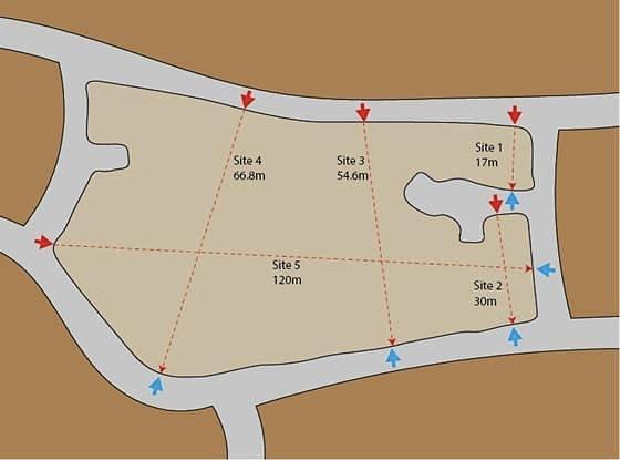
The trans illumination experiments were conducted 700m below the surface within the historical mined-out workings of the Pend Oreille zinc and lead mine, Washington State, USA. Radar pulses were sent and recorded in the access tunnels through a limestone pillar along five paths through distances of 16m, 26m, 55m, 67m, and 121m as indicated in Fig. 1. We generated a directional broadband pulse where indicated by the red arrows, aimed towards the receiver (blue arrow). To correct for possible aiming errors, data were recorded at 11 locations on a 20m range around the target, and the largest signal was selected. Each trace was replicated 500 times and stacked (averaged) to increase the signal to noise ratio.
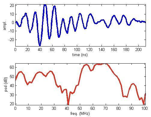
The directional radar pulse was emitted and recorded using equipment provided by Adrok Ltd (Stove et al., 2012). We recorded the pulse in air and show its temporal and spectral shape in Fig 2. The dominant frequency components are at 55 − 70MHz, 30MHz, 20MHz, and 3MHz. We verified the directionality of the pulse by additional measurements in air.
The goal of the second experiment was to determine if reflections from the low frequency component of the pulse could be detected and distinguished from clutter at a large depth of 350m (i.e., 700m two-way travel). The second experiment was performed in the same mine at a location 350m under the Pend Oreille river. The pulse was aimed upwards through the ceiling of the tunnel and the receiver was placed at a distance of 1m from the receiver and as before, 500 traces were recorded.
Results
Experiment 1
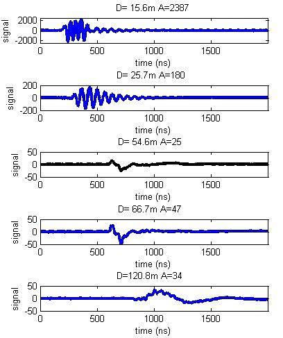
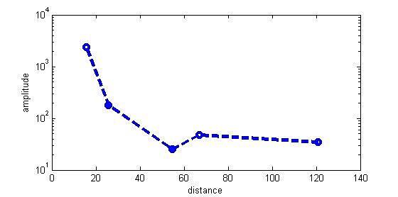
The measured transmitted pulses through the 5 paths are depicted in Fig. 3 where we also indicate the maximum amplitudes, which are plotted on a logarithmic scale in Fig. 4. The third scan at D = 55m is weaker than all the others which we believe is due to an aiming error, resulting in a partial scattering off the cavity which is visible on the right in Fig. 1.
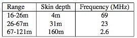
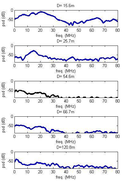
It is clear that the losses do not follow an exponential decay law (which would be a straight line), and that the shape as well as the amplitude of the pulse changes with penetration distance, with only a ≈ 3MHz pulse surviving at the largest distance. The most likely explanation is that the high frequency components get stripped off early on, resulting in a rapid decrease in amplitude at first, after which the low frequency component decays much slower. This effect can also be seen in the power spectral densities of the returns which are shown in Fig. 5. Discarding the third measurement, we compute the effective skin depths at several depths which are listed in Table 1. (The third column will be explained below.)
To put these numbers into a physical modeling context we implemented a time-domain finite volume simulation of Maxwell’s equations in a medium described by a relative permittivity εr(x), a static conductivity σ and a Debye polarization model (Debye, 1929) with relaxation time τ to model the high frequency losses. Parameters are assumed to be constant in time but can depend on location. It is well known that polarization losses are described more accurately with the ColeCole model (Cole and Cole, 1941, 1942), but that model does not lend itself to a time-domain numerical solution. Restricting the model to propagation in one direction, we obtain the following system of partial differential equations:
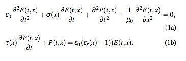
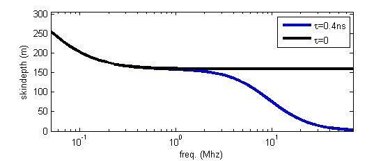
The vacuum permittivity and permeability are ε0 = 8.85 × 10⁻¹² F/m and μ0 = 4π × 10−7 H/m. For constant material parameters we fitted these to match the data and obtained a reasonably good match with εr = 5.7, σ = 0.075mS/m, and τ = 0.4ns. The relative permittivity is obtained directly from the measured travel time of the pulse over 121m. Next we obtained σ by matching the skin depth at 3MHz to Table 1. To obtain τ we assumed the 4m skin depth is governed by the 60 − 70MHz component of the pulse, and the 31m skin depth by the 20 − 30MHz component. The skin depth can be obtained by standard means from (1) by solving the dispersion relation. In Fig. 6 we plot the theoretical skin depth as a function of frequency with and without polarization losses. We see the familiar low frequency ≈ 1/√σ f behaviour below 100kHz, the curve then flattens out and the polarization losses start to dominate around 10MHz. We have indicated in the last column of Table 1 the frequencies corresponding to the skin depths at various ranges.
Experiment 2
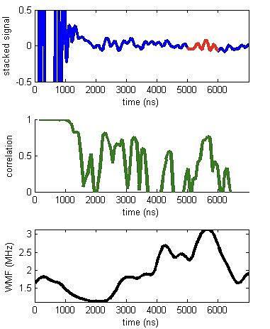
The results from the upward looking scan are depicted in Fig. 7 Assuming the same relative permittivity as was measured in Experiment 2, the reflection from the river should be located at 5570ns and we do indeed see what appears to be a reflection at 5300ns in the stacked trace. This corresponds to a (harmonic) mean relative perimittivity of 5.2, which is a bit smaller than the value 5.7 obtained from Experiment 1.
To further validate this observation we computed the mean correlation between the individual traces and note the large peak at the correct time, indicating there is definitely information there. As a third check we computed the amplitude weighted mean frequency (WMF). The WMF was computed by performing a continuous wavelet transform using the Gabor (or Morlet) wavelet Gabor (1946), and computing the mean of the frequency, weighted by the absolute value of the wavelet coefficient. We observe it peaks at the value 3MHz, corresponding to the low frequency component of the transmitted pulse, at the correct time.
To check that these results do not contradict theoretical expectations we performed a time-domain numerical simulation of (1), and repeated Experiment 2 in simulation. The PDE system was discretized with a finite volume method, using a fourth order discrete Laplacian in space, a leap-frog algorithm to advance time for E, and a backwards Euler method to time step P (see for example Ascher (2008)). Unlike most EM simulations, we do not have sources and boundary conditions, but instead have an initial value problem with P(t = 0, x) = 0 and E(t = 0,x) and ∂E(t,x)|t=0 set to the measured pulse shape ∂t (see Fig 2) moving in air at the speed of light towards the rock layer.
The spatial domain consists of an air section where the pulse is initially placed, a ground section ranging from 0 − 350m with a spatially variable relative permittivity, and a water layer of 9m with a relative permittivity of 81. The physical domain is padded with 200m absorbing layers using the perfectly matched layer (Berenger, 1994) method to extinguish waves and avoid spurious reflections.
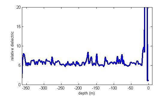
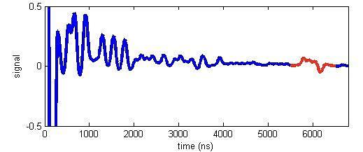
We set the conductivity and Debye relaxation time in rock to the values obtained from Experiment 1 (σ = 0.075mS/m, τ = 0.4ns) and the relative permittivity was set to the profile depicted in Fig. 8. The profile has irregular fluctuations superimposed on an average of 5.7 which was obtained from Experiment 1, and represents our best guess for a semi-realistic constitutive model with various irregularities. The simulated trace is shown in Fig. 9. We observe that the reflection from the water (highlighted in red) is apparent and not obscured by clutter. Comparing with the real data in Fig. 7 we see that the simulated reflected pulse has a different shape, indicating the actual absorption mechanism is more complicated than our model, which is not surprising as the Debye model for losses is not very realistic, and there are most likely variations in absorption characteristics which we do not model. With the data we have obtained from the present study it is not possible to be more precise. The simulated pulse arrives 270ns after the measured pulse because our estimate of the relative permittivity was off by 9%, as noted before.
Despite these discrepancies we believe the simulation shows that there is no theoretical objection to measure a reflection through 350m of rock.
Discussion
The results from the two experiments describe here as well as the numerical model simulation suggest that the exploration depth of pulsed radar can be increased significantly by including a low frequency component. Our data suggests the high losses of GPR in the 10 − 1000MHz range are due to polarization effects, rather than conductivity losses. The conductivity we found to be consistent with our data was 0.075mS/m. It would be desirable to confirm this value with independent measurements. Values for limestone conductivity reported in the literature vary widely, for example (Telford et al., 1990) quotes a range of 10−7 − 2 × 10⁻² S/m. The actual value depends on complicated and not fully understood details of how pore water is embedded in the rock, and which solvents are present in the solution. See for example Revil (2013).
For example Scho ̈n (2004) quotes values from σ = 10−2S/m (wet) to σ = 10−5S/m (dry) with permittivity values of εr = 11 (wet) to εr = 6 (dry). This suggest a rather low water content of the rock in our study.
If these results hold for other rock types, deeply penetrating radar scanning can potentially become an attractive geophysical exploration technique in selective environments where there is no highly conductive near-surface layer, or where this layer is thin enough to penetrate. We believe that these experiments are encouraging and warrant further investigations.
Acknowledgments
We would like to thank Teck Washington Incorporated for providing access to the Pend Oreille mine, and Uri Ascher for help with the numerical solution of the model equations.
- Ascher, U., 2008, Numerical Methods for Evolutionary Dfer- ential Equations: SIAM.
- Berenger, J., 1994, A perfectly matched layer for the absorp- tion of electromagnetic waves: Journal of Computational Physics, 114, 185–200.
- Cole, K. S., and R. H. Cole, 1941, Dispersion and Absorp- tion in Dielectrics I. Alternating Current Characteristics: J. Chem. Phys., 9, doi: 10.1063/1.1750906.
- 1942, Dispersion and Absorption in Dielectrics II. Direct Current Characteristics: J. Chem. Phys., 10, doi: 10.1063/1.1723677.
- Debye, P., 1929, Polar Molecules: Chemical Catalogue Com- pany.
- Gabor, D., 1946, Theory of communication: Journal of the Institute of Electrical Engineers, 93, 429–457.
- Jol, H. M., 2009, Ground Penetrating Radar Theory and Ap- plications: Elsevier.
- Revil, A., 2013, Effective conductivity and permittivity of un- saturated porous materials in the frequency range 1 mHz- 1GHz: Water Resources Research, 49, 306–327.
- Scho ̈n, J. H., 2004, Physical Properties of Rocks, Volume 8: Fundamentals and Principles of Petrophysics: Elsevier. Stove, G., J. McManus, M. J. Robinson, G. Stove, and A.
- Odell, 2012, Ground penetrating abilities of a new coherent radio wave and microwave imaging spectrometer: Interna- tional Journal of Remote Sensing, 34, 303–324.
- Telford, W. M., L. P. Geldart, and R. E. Sheriff, 1990, Applied Geophysics: Cambride Univerity Press.